A Brief Introduction to Ruthroff Transmission Line Transformers – Technical Articles

The broadband capabilities of transmission line transformers make them highly useful in RF applications. These transformers come in a variety of configurations, depending on the type, number, and arrangement of the transmission lines used. Previous articles in this series explored the Guanella 1:1 and Guanella 1:4 baluns, two classic circuits first presented by Gustav Guanella in 1944.

15 years after that, a paper by C. L. Ruthroff introduced a new class of broadband transmission line transformers to the world. In this article, we’ll gain a basic understanding of the Ruthroff transformers—both balanced-to-unbalanced and unbalanced-to-unbalanced—by conducting a simplified analysis.

The Ruthroff 1:4 Unbalanced-to-Unbalanced Transformer

Figure 1 shows a configuration we’re already familiar with—the Guanella 1:4 balun, which incorporates two transmission lines.

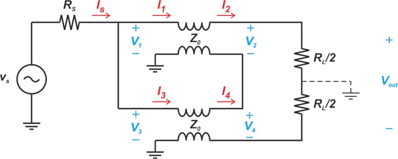
Figure 1. The Guanella 1:4 balun.

When the balun function isn’t required, we can rearrange a single bifilar coil to provide a 1:4 impedance transformation ratio. Figure 2 depicts this circuit, known as the Ruthroff 1:4 unbalanced-to-unbalanced transformer. You may also see it referred to as the Ruthroff 1:4 “unun,” echoing how we abbreviate “balanced-to-unbalanced transformer” as “balun.” I—like many others—find the term “unun” inelegant and unattractive, and so choose not to use it.

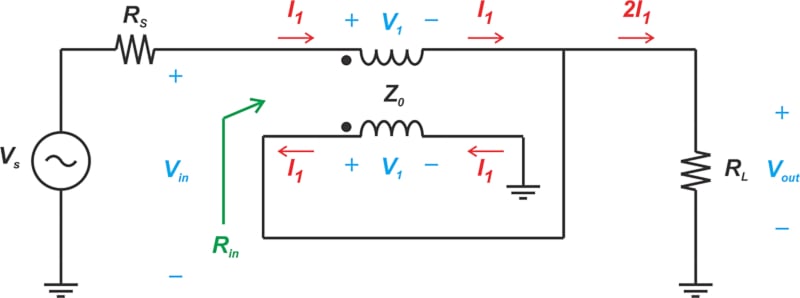
Figure 2. The Ruthroff 1:4 unbalanced-to-unbalanced transformer.

Using the lumped inductor method introduced in the preceding article, let’s analyze this circuit.

Assume that the current through the upper winding is I₁ and the voltage drop across it is V₁. Due to the transformer action, a voltage difference of V₁ is also impressed across the lower winding, and a current of I₁ flows through this winding in the indicated direction. The current through the load is therefore equal to 2I₁.

Since the lower winding is in parallel with the load, the voltage across the load (V_out) is also equal to V₁. The voltage at the input terminal can easily be determined by summing the voltage across the upper winding and the load resistor, leading to:

$$V_{in}~=~V_{1}~+~V_{out}~=2V_{1}$$

Equation 1.

For the load resistor (R_L), Ohm’s law defines another relationship between V₁ and I₁:

$$R_L ~=~ frac{V_{out}}{2I_1}~=~ frac{V_1}{2I_1}$$

Equation 2.

We now express the input resistance (R_in) in terms of V₁ and I₁, using Equation 2 to simplify it:

$$R_{in} ~=~ frac{V_{in}}{I_1}~=~frac{2V_1}{I_1}~=~4R_L$$

Equation 3.

The equivalent input resistance is four times the load resistance. To analyze the above circuit more quickly, keep the following in mind:

• The input voltage is equal to the sum of the voltage drops across the two windings (V_in = V₁ + V₂).
• Due to the transformer action, the two voltage drops are equal (V₁ = V₂).
• The output voltage is equal to the voltage drop across one of the windings (V_out = V₁ = V₂).
• The input voltage is therefore two times the output voltage (V_in = V_out + V_out = 2V_out).
• A lossless network that changes the voltage by a factor of two produces a 1:4 impedance transformation ratio.

Like the Guanella configurations, the Ruthroff transformers don’t provide DC isolation. Both of these transformer types ideally induce zero net flux in the core material during odd-mode excitation. This significantly reduces the frequency-dependent hysteresis losses of the core, which is often what sets the upper end of the transformer’s bandwidth.

Figure 3 demonstrates a coaxial implementation of the Ruthroff circuit. Note that the coaxial line would usually be loaded with ferrite beads, though these aren’t shown in the figure.

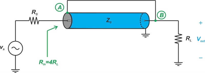
Figure 3. A coaxial realization of the Ruthroff 1:4 unbalanced-to-unbalanced transformer.

For minimal leakage inductance, the distance between points A and B should be as short as possible. This might require bending the line to get the connection points close together. Also note that, in the Ruthroff transformer, the characteristic impedance of the line (Z₀) is equal to the geometric mean of the input and output impedances:

$$Z_0 ~=~ sqrt{R_S R_L}$$

Equation 4.

The Ruthroff 1:4 Balun Transformer

Figure 4 shows the Ruthroff 1:4 balun. Like the unbalanced-to-unbalanced transformer, it’s built around a single bifilar coil.

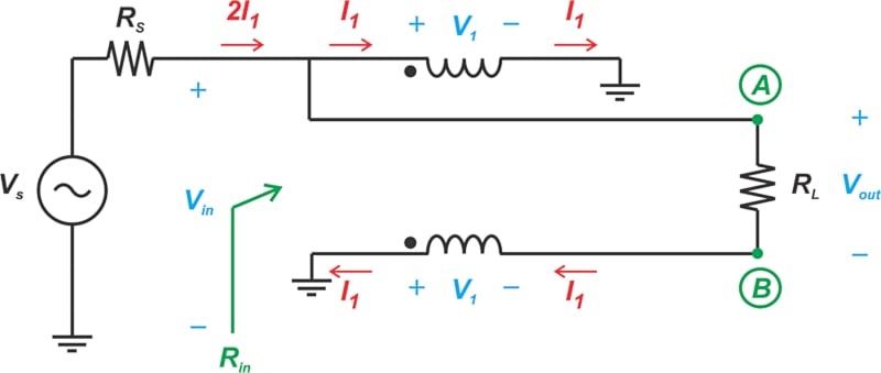
Figure 4. The Ruthroff 1:4 balun.

Once again, the same voltage appears across the two windings due to the transformer action. By grounding the appropriate terminals of the windings, voltages with opposite polarities are produced at the load resistor terminals. In other words, nodes A and B have the same voltage with opposite polarities.

It’s easy to see from the circuit diagram that the input voltage is equal to the voltage drop across one winding (V_in = V₁), whereas the voltage across the load is V_out = 2V₁. The circuit therefore doubles the input voltage, producing a 1:4 impedance transformation ratio. Because the load isn’t grounded at either end, the output is a balanced signal.

Up Next

Compared to the Guanella transformers, the Ruthroff configurations provide a relatively lower bandwidth. We’ll discuss this more in the next article of this series, when we conduct a more rigorous analysis of these circuits. We’ll also examine some simple modifications that, when applied, can improve the Ruthroff transformers’ bandwidths.

All images used courtesy of Steve Arar