
A gyroscope is a sensor that measures the rate of rotation of an object. The workings of gyroscopes can be mysterious to many engineers.
With that in mind, as well as being inspired by an article from Analog Devices, this article attempts to give a more detailed explanation of the theory behind the MEMS vibratory gyroscopes. Since a thorough analysis can be math-intensive, we’ll try to consider a special orientation of the sensor to simplify the discussion as much as possible.
Position of a Rotating Object Using a Polar Coordinate System
The position of a rotating object can be more easily described using a polar coordinate system. Assume that, as shown below in Figure 1, the object is always in the XY plane.
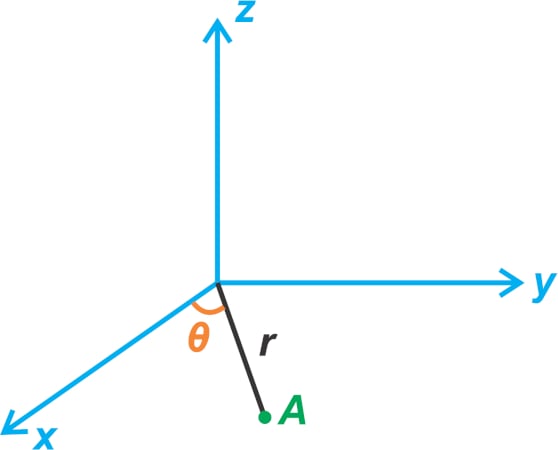
Figure 1. An example object on an XYZ plane.
As θ changes, point A rotates about the z-axis. You may recall from math classes that the unit vectors $$hat{r}$$ and $$hat{theta}$$ are defined for a polar coordinate system, as shown in Figure 2 to uniquely specify a point in the XY plane.
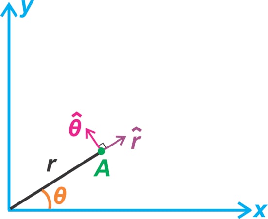
Figure 2. An example polar coordinate system.
Since the object is assumed to be always in the XY plane, a 2D representation is used in the above figure. The position of the object, $$overrightarrow{P_A}$$, can now be described as:
$$overrightarrow{P_A}=rhat{r}$$
Equation 1.
The above equation might be confusing as it doesn’t make any reference to the angle θ. However, note that the unit vector $$hat{r}$$ is not a fixed vector and its orientation depends on θ.
The Velocity of a Rotating Object—Finding the Time Derivative
The object velocity can be found by taking the time derivative of the position vector. Applying the product rule to Equation 1, we obtain:
$$overrightarrow{V_A}=frac{text{d}}{text{d}t} big (overrightarrow{P_A}big ) = frac{text{d}r}{text{d}t}hat{r}+rfrac{text{d}hat{r}}{text{d}t}$$
Equation 2.
The first term takes into account an obvious point: if we keep θ constant, we can still change the object’s position by changing its distance from the origin by Δr, as shown in Figure 3. In this case, the velocity should have a radial component, i.e. in the direction of $$hat{r}$$.
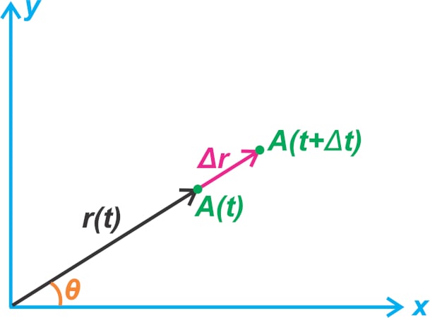
Figure 3. The change in the object’s position by changing its distance.
The second term in Equation 2 takes into account the fact that the object’s position can change due to rotation, even if the distance from the origin is constant. Remember that, although $$hat{r}$$ has a length of 1, its orientation depends on θ and can change with time. Figure 4(a) shows how the position changes if we keep r constant and increase the angle by Δθ.
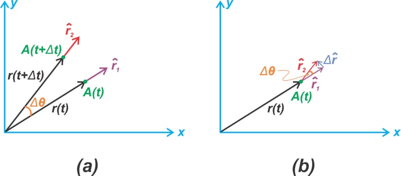
Figure 4. Example of how the position changes if r is constant and angle increases by Δθ (a) and finding that change (b).
To find the change in $$hat{r}$$, we can draw $$hat{r_2}$$ from the origin of $$hat{r_1}$$ as shown in Figure 4(b). The angle between these two vectors is Δθ. Assuming that Δθ is very small, simple geometry formulas give the magnitude of change in $$hat{r}$$ as:
$$lvert Delta hat{r} rvert=hat{r_2}-hat{r_1} approx lvert {hat{r_1}} rvert Delta theta = Delta theta$$
Dividing both sides by the time interval Δt, in which the change occurs and taking the limit, we obtain:
$$lvertfrac{text{d}hat{r}}{text{d}t}rvert= lim_{Delta t rightarrow 0} frac{lvert Delta hat{r} rvert}{Delta t} = lim_{Delta t rightarrow 0} frac{Delta theta}{Delta t} = frac{d theta}{dt}$$
This gives us the magnitude of the derivative. Since we are working with vector values, we also need to find the vector direction. As you can see from Figure 4(b), with a very small value of Δθ, $$frac{text{d}hat{r}}{text{d}t}$$ is in the direction of $$hat{theta}$$.
Thus, we have:
$$frac{text{d}hat{r}}{text{d}t}=frac{text{d}theta}{text{d}t}hat{theta}$$
Equation 3.
$$overrightarrow{V_A}= frac{text{d}r}{text{d}t}hat{r}+rfrac{text{d}theta}{text{d}t}hat{theta}$$
Equation 4.
Acceleration of a Rotating Object
Taking the derivative of Equation 4, we can find the object acceleration as:
$$overrightarrow{A_A}=frac{d}{dt} Big ( frac{text{d}r}{text{d}t}hat{r}+rfrac{text{d}theta}{text{d}t}hat{theta} Big )$$
Equation 5.
Applying the product rule to the first term inside the parentheses, we obtain two terms:
$$frac{d}{dt} Big ( frac{text{d}r}{text{d}t}hat{r} Big ) = frac{d^2r}{dt^2}hat{r} + frac{dr}{dt}frac{d hat{r}}{dt}$$
Substituting Equation 3 into the above equation, we arrive at:
$$frac{d}{dt} Big ( frac{text{d}r}{text{d}t}hat{r} Big ) = frac{d^2r}{dt^2}hat{r} + frac{dr}{dt}frac{text{d}theta}{text{d}t}hat{theta}$$
Equation 6.
The first term on the right side of this equation is the mathematical expression of an obvious point. It states that, for a given θ, the object can have radial acceleration if the second derivative of r is non-zero. However, the second term of the equation reveals an interesting phenomenon: if the object’s distance from the origin r changes while it rotates around the z-axis, the object experiences acceleration in the direction of $$hat{theta}$$.
Vibratory gyroscopes use this phenomenon to measure angular velocity by incorporating a mass that continuously vibrates. When the sensor rotates, the mass deflects depending on the rate of change of θ. By measuring the mass deflection, it is possible to determine the angular velocity of the object. We’ll discuss this in greater detail below.
However, what about the second term of Equation 5?
Differentiating this term gives us three acceleration terms:
$$frac{d}{dt} Big ( rfrac{text{d}theta}{text{d}t}hat{theta} Big ) = frac{dr}{dt}frac{dtheta}{dt}hat{theta}+r frac{d^2theta}{dt^2}hat{theta}- r big( frac{dtheta}{dt} big ) ^2 hat{r}$$
Equation 7.
The first term again leads to the phenomenon we discussed above: if the object’s distance from the origin changes while it rotates around the z-axis, the object experiences acceleration in the direction of $$hat{theta}$$.
The second term also gives a tangential acceleration component; however, this term is created only when the second derivative of θ is non-zero. In practical applications of gyroscopic sensors, this term is assumed to be zero, which is why we’ll ignore this term in the rest of the article.
The third term is also a radial component and is the centripetal acceleration that a rotating object experiences. By substituting our findings into Equation 5, we obtain the following total acceleration:
$$overrightarrow{A_A}= Big ( frac{d^2r}{dt^2} – r big( frac{dtheta}{dt} big ) ^2 Big ) hat{r} + Big ( 2frac{dr}{dt}frac{text{d}theta}{text{d}t} Big ) hat{theta}$$
Equation 8.
Insight Into the Equations
The tangential term in Equation 8 is key to the operation of a vibratory gyroscope. Let’s more closely examine how this term is created. Figure 5 shows the trajectory of a bead that moves along the spoke of a rotating wheel.
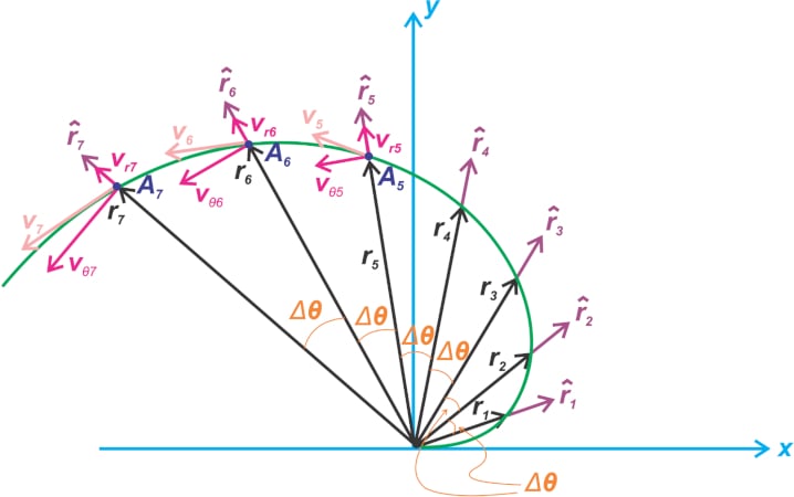
Figure 5. An example showing the trajectory of a bead along a rotating wheel spoke.
The bead moves along the spoke with a constant speed of u, i.e. the radial distance from origin |r| is equal to ut. The angular velocity of the wheel is shown as:
$$frac{dtheta}{dt}$$
The angular velocity is constant and equal to ⍵. The black vectors show the position of the bead after consecutive time intervals of Δt which corresponds to a change of Δθ in the angle. From Equation 4, we know that the velocity vector at a given time has a radial component of:
$$v_{r}=frac{dr}{dt} = u $$
As wells as a tangential component of:
$$v_{theta} = rfrac{dtheta}{dt} = romega$$
Figure 5 shows these velocity components for positions A5, A6, and A7. In our example, the magnitude of the radial component is constant but what about the tangential component?
Since ⍵ is constant, the tangential component of velocity increases with r. In other words, as we move further away from the origin, the bead has to travel a longer distance for a given time interval and Δθ. You can clearly see this by comparing the distance between the consecutive position vectors.
Another question is how fast can the tangential velocity change due to this phenomenon?
For a given ⍵, the rate of change of the tangential velocity, which gives a tangential component of acceleration, is equal to the rate of change of r. Therefore, one component of the tangential acceleration is given by:
$$A_{1} = frac{dr}{dt} times omega = frac{dr}{dt} times frac{dtheta}{dt}$$
This gives us the first term on the right side of Equation 7. Overall, this acceleration component is created by changes in the magnitude of the tangential component of velocity $$v_{theta} = romega$$. There is another mechanism that leads to a tangential acceleration component: changes in the direction of the radial component of velocity:
$$v_{r} = frac{dr}{dt} = u$$
Although the magnitude of this term is constant in our example, its direction is a function of time. You can see from Figure 5 how the direction of the unit vector $$hat{r}$$ rotates with time. We know from Equation 3 that the rate of change of $$hat{r}$$ is equal to:
$$frac{dtheta}{dt}hat{theta}$$
Therefore, changes in the direction of the radial velocity $$v_{r}=frac{dr}{dt}$$ leads to the second tangential component of acceleration:
$$A_{1} = V_{r}timesfrac{d}{dt}(hat{r})=frac{dr}{dt}timesfrac{dtheta}{dt}$$
Thus, the total tangential component of acceleration for an object rotating at an angular velocity of ⍵ is given by:
$$A_{theta} = 2 times frac{dr}{dt} times frac{dtheta}{dt} = 2 times frac{dr}{dt}times omega$$
Basic Structure of a MEMS Gyroscope
Figure 6 shows the basic structure of a vibratory gyroscope.
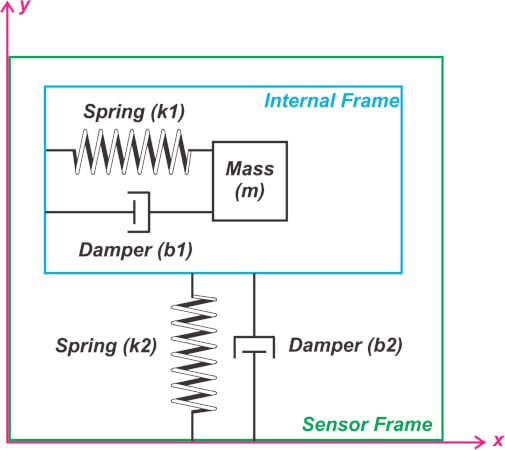
Figure 6. An example structure of a vibratory gyroscope.
The mass (m) is connected to the “internal frame” through a damper-spring structure. Moreover, an actuator controlled by a positive feedback system (not shown above) is used to drive the mass into a harmonic oscillation. The feedback system guarantees that the mass is kept in a regulated continuous oscillation along the x-axis, as shown in the figure. Moreover, the internal frame is connected to the “sensor frame” through a second damper-spring structure at 90° relative to the mass oscillation direction. This configuration allows the internal frame to be able to move in the y-axis direction when a force is present in this direction.
As we’ll see in the next section, the structure shown in Figure 6 can detect angular velocity when the sensor is rotated about an axis perpendicular to the XY plane depicted in the figure.
How Does a Vibratory Gyroscope Work?
Assume that, as shown in Figure 7, the gyroscope is fixed to a platform that rotates in a counterclockwise direction.
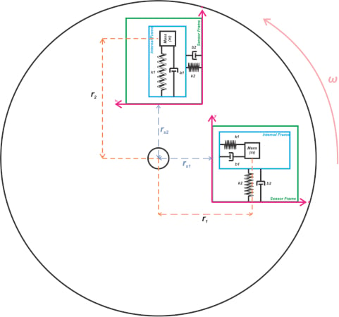
Figure 7. A gyroscope on a fixed platform that rotates counterclockwise.
The figure shows the sensor at two different instants. Although the distance of the sensor package from the center of the platform is fixed, we know that the mass distance changes from r1 to r2 due to its oscillation in the x-direction of the sensor frame. In this example, the mass distance increases r2 > r1.
Similar to the bead example depicted in Figure 5, the proof mass experiences a tangential acceleration in the positive direction of the sensor y-axis. In the y-direction, the proof mass is rigidly connected to the internal frame. Therefore, the same acceleration is also applied to the internal frame. The internal frame; however, initially tends to stay at rest, which changes the relative position of the internal frame with respect to the sensor frame.
This relative displacement, proportional to the input angular velocity, can be measured by several means such as the capacitive sensing approach that we discussed in a previous article about accelerometers. Thus, gyroscopes can be described as a resonator along the drive direction and as an accelerometer along the sensing direction.
To see a complete list of my articles, please visit this page.